Occupancy models with INLA crash when too many visits per period and sites

Summary

We have coded occupancy models using the very nice available tutorials and they have been working fine so far. However, when using datasets with too many visits per year and site we observe that INLA crash almost systematically. Our large number of visits per year is linked to the fact that we use opportunistic dataset and not standardised surveys. Since repeated visits are key in occupancy models (the more replication, the better the estimation of detection probability), we are currently blocked by the fact models crash when including too many visits. Below you will find a code allowing to reproduce that bug. This code simulate datasets with different levels of replication and assess the likelihood of crashing when running INLA occupancy models.

The occupancy model

The occupancy model we will run here is a very simple model, with just a baseline detection probability in the observation model and a baseline occupancy in the state model.

State model

\[z_{it} \sim \mathrm{Bernoulli}(\psi_{it})\] \[\operatorname{logit}(\psi_{it}) = \beta_0 + \omega_i\] Observation model
\[y_{itj} \mid z_{it} \sim \mathrm{Bernoulli}(z_{it}\times p_{itj})\] \[ \operatorname{logit}(p_{itj}) = \alpha_0 \]

Here, \(z_{it}\) denotes the occupancy state in site \(i\) for year \(t\). \(\psi_{it}\) is the associated occupancy probability defined on the logit scale as a linear function of an intercept (\(\beta_0\)) and \(\omega\), a spatial Gaussian random field describing the spatial structure in the data.

The response \(y_{ijt}\) is the detection/non-detection data for site \(i\), year \(t\) and visit \(j\), given \(z_{it}\). The detection probabilities \(p\) are defined on the logit scale as a linear function of \(\alpha_0\) (Intercept).

The problem

In our study case we have a maximal number of visits per year and site, K (\(j=1,...,K\)). Let’s imagine our data are aggregated at month level, the maximal number of visits per year and site is \(K=12\). However, since not all sites are monitored every months every year, then the number of realized visits (\(K_{obs}\)) depends on the year and site combination. In our simulations, we varied the average number of realized visits (\(\overline{K}_{obs}\)).

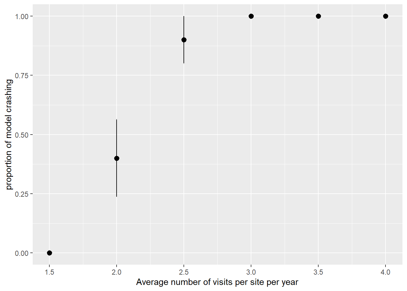
When the average number of realized visits, \(\overline{K}_{obs}\), increased, the probability of the model to crash sharply increased to reach one around \(\overline{K}_{obs} = 3\). Below you will find a code allowing to reproduce that bug.

R and INLA versions

Loading packages and showing R and INLA versions:

library(data.table)
library(INLA)
library(fmesher)
library(raster)
library(dplyr)
library(sf)
library(terra)
library(spatstat.geom)
library(MASS)
library(ggplot2)

R.version

               _                                
platform       x86_64-w64-mingw32               
arch           x86_64                           
os             mingw32                          
crt            ucrt                             
system         x86_64, mingw32                  
status                                          
major          4                                
minor          5.2                              
year           2025                             
month          10                               
day            31                               
svn rev        88974                            
language       R                                
version.string R version 4.5.2 (2025-10-31 ucrt)
nickname       [Not] Part in a Rumble           

packageVersion("INLA")

[1] '26.5.21'

Simulating data

We first define an abitrary spatial domain to simulate data across that domain.

ART: Approximate Running Time

# Define spatial domain
win <- owin(c(0,10), c(0,10))
nc <- 20
nr <- 20 #20*20 means 400 sites

Domain <- rast(nrows=nr, ncols=nc,
               xmax=win$xrange[2],xmin=win$xrange[1],
               ymax = win$yrange[2],ymin=win$yrange[1])

values(Domain) <- 1:ncell(Domain)
names(Domain)="cell_id"

We then define a function to simulate data, according to the basic assumption of our occupancy model (stable occupancy and detectability across time, etc.).

This function has the following arguments:

Parameter	Meaning
nT	number of years
nM	maximal number of repeated visits, let’s say 12 if data are aggregated at month level
prop_sampled	proportion of sites sampled each year
occ_0	initial occupancy probability
trend	growth rate: <1 means declining, 1 means stable, >1 means increasing
det_prob	species detection probability
nrepli	number of independent datasets to generate
nrep_avg	average number of repetited visits (1 repetition means 2 visits in a year per site)

simulate_data=function(nT, nM,prop_sampled, occ_0, trend, det_prob, nrepli, nrep_avg){ 
  
  det_tab_list=list()
  for(repli in 1:nrepli){ #loop over the number of datasets to generate

    #yearly average occupancy (if trend)
    occs <- boot::inv.logit(boot::logit(occ_0)+log(trend)*(0:(nT-1))) #yearly occupancy
    occs_logit <- boot::logit(occs)
    
    #generate species occupancies with spatial autocorrelation
    distances <- as.matrix(dist(crds(Domain)))
    cov_mat <- as.matrix(exp(-distances))
    #generate spatially autocorrelated deviation to the mean:
    random_field <- mvrnorm(1,mu=rep(0,nr*nc),cov_mat)
    #generate spatio-temporal occupancy values:
    occ_tab <- data.frame(cell_id=rep(values(Domain$cell_id),nT),
                         x=rep(crds(Domain)[,1],nT),y=rep(crds(Domain)[,2],nT),
                         proba=boot::inv.logit(random_field + rep(occs_logit, each=nr*nc) - mean(random_field)),
                         year=rep(1:nT,each=nr*nc))
    #draw real occupancy values:
    occ_tab$occ <- rbinom(nr*nc*nT,1,occ_tab$proba)
    
    #draw species detection
    det_tab = NULL
    for(i in 1:nT){ # a loop over years
      
      bidon <- subset(occ_tab,year==i) #take only the year we focus on
      
      #sample randomly some sites
      sample_sites <- sample(1:nrow(bidon),round(prop_sampled*nrow(bidon)),replace=FALSE)
      #take only the sites we focused on
      bidon <- bidon[sample_sites,]
      
      bidon$nrep <- 1+rnbinom(length(sample_sites),mu=nrep_avg,size=2) #each sampled site is visited at least once + an undefined number of repetition
      
      bidon$nrep[bidon$nrep>=nM]=nM #if number of repetition exceed maximal number of repetition then truncate
      
    
          
        #replicate each site line for each visit
        det_tab1 <- do.call("rbind",lapply(1:nrow(bidon),
            function(x){do.call("rbind",replicate(bidon$nrep[x], bidon[x,],simplify=FALSE))}))
        #add the ID associated with each visit (not important here but it is in case we include covariates)
        # if we assume visits have the same probability to be realized (a visit = a month)
        det_tab1$visit_n=unlist(sapply(bidon$nrep,function(x){sample(1:nM,x,replace=F,prob=rep(1/nM,nM))}))
        #generate detection 
        det_tab1$detection=det_tab1$occ*rbinom(nrow(det_tab1),1,det_prob)
        
        #storing parameters:
        det_tab1$nrep_avg=nrep_avg
        det_tab1$repli=repli
        
        #combine across years
        det_tab=rbind(det_tab,det_tab1)
        
    }
    det_tab_list[[repli]]=det_tab
  }
  
    return(det_tab_list)
}

We will use that function to simulate several datasets with different number of repeated visits, keeping other parameters fixed:

############## FIXED PARAMETERS
nT <- 10 #number of years
nM <- 12 #maximal number of visits, let's say 12 if data are aggregated at month level
prop_sampled <- 0.2 #proportion of sites sampled each year

#species occupancy probabilities
occ_0 <- 0.5 #initial occupancy probability
trend <- 1.0 #growth rate: <1 means declining, 1 means stable, >1 means increasing

#species detection
det_prob <- 0.2 #species detection probability


nrepli <- 10 # generate 5 independent datasets perparameter condition

############## VARYING PARAMETER
nrep_avg_vec=seq(0.5,3,by=0.5) #average number of sampling repetition (1 repetition means 2 sampling events in a year)


############## SIMULATING DATA
list_data=lapply(nrep_avg_vec,function(x){simulate_data(nT, nM,prop_sampled, occ_0, trend, det_prob, nrepli, x)})

Implementing occupancy models with INLA

We coded a function that run occupancy models, following the following tutorials: https://ecol-stats.github.io/Occupancy-Models-in-INLA-/website/docs/.

Since we did not include any covariates for detection, only an intercept, the matrix of detection covariates (X_det) is filled only with 1 and has \(M\) rows and \(K\) columns, where \(M\) is the number of \(sites \times year\) combinations and \(K\) is the number of visits:

\[ X_{det} = \begin{matrix} 1 \\ \vdots \\ M \end{matrix} \overbrace{\begin{pmatrix} 1 & \dots & 1 \\ \vdots & \vdots & \vdots \\ 1 & \dots & 1 \end{pmatrix}}^{\begin{matrix} 1 & \dots & K \end{matrix}} \]

max_fd <- function(x){ifelse(length(x)>0,max(x),NA)} #personnalized function, return max if it has element, NA otherwise

# a function running INLA occupancy models

run_occupancy_model=function(det_tab){
  
  setDT(det_tab)
  
  #create the big matrix of number of records per sampling events for all species (work with data table to speed up and save memory):
  matrix_spat <- dcast(det_tab,cell_id+x+y+year~paste0("V",visit_n),value.var="detection",fun.aggregate=max_fd)
  
  ncells <- length(matrix_spat$cell_id %>% unique)  # number of cells in the whole area
  
  # Convert to sf
  space_data_sf <- vect(unique(matrix_spat[,c("x","y","cell_id")]),geom=c('x','y'),crs="EPSG:4326")
  
  ########### creat the mesh
  boundary_sf = st_bbox(space_data_sf) %>%
  st_as_sfc() %>% st_as_sf()
  
  mesh <- fm_mesh_2d(loc.domain = st_coordinates(boundary_sf)[,1:2],
                max.edge = c(15, 30))
  
  spde <- inla.spde2.pcmatern(mesh = mesh,
                          prior.range = c(100, 0.5),
                          prior.sigma = c(1, 0.5))
  
  t_points <- unique(matrix_spat$year)# unique time points
  
  # index set; "spatialfield" is the name used in the model formula
  iset_sp <- inla.spde.make.index(name = "spatialfield", 
                            n.spde =  spde$n.spde,
                            n.group = length(t_points))
  # projection matrix using the coordinates of the data and time index
  A_sp <- inla.spde.make.A(mesh = mesh,
                     loc = as.matrix(matrix_spat[,c("x","y")]),
                     group = matrix_spat$year)
  
  Y_mat <- matrix_spat %>%
  dplyr::select(num_range("V",sort(unique(det_tab$visit_n)))) %>% 
  as.matrix()
  
  #detection covariates in the good format (only one intercept):
  matrix_spat$intercept=1
  X_det <- matrix_spat[,rep("intercept",length(unique(det_tab$visit_n))),with=FALSE] %>% as.matrix()
  
  #occupancy covariates
  X_cov <- matrix_spat %>%
  dplyr::select(c(year,cell_id))
  
  
  stk <- inla.stack(data=list(Y = Y_mat,  X = X_det),
              A=list(A_sp,1),
              effects=list(c(list(Int_occ=1), #the Intercept
                             iset_sp),  #the spatial index
                           #the covariates
                           as.list(X_cov)),
              tag='spat')
              
  formula_spat <- inla.mdata(Y,X) ~ -1 + Int_occ +
    f(spatialfield,
    model=spde)
  
  #running the model with a trycatch to avoid errors breaking the loop
  obj <- tryCatch({model_spat <- inla(formula_spat, #the formula
           data=inla.stack.data(stk),  # the data stack
           family= 'occupancy',   # model likelihood
            control.predictor=list(A=inla.stack.A(stk),compute=TRUE),
            control.family = list(control.link = list(model = "logit"),
                link.simple = "logit"),verbose=F)},error=function(x){return(NA)})
  
  rest <- data.frame(repli=unique(det_tab$repli),
                  nrep_avg=unique(det_tab$nrep_avg),
                  run_success=ifelse(class(obj)=="inla",1,0)) #if model crashed then put 0, if model runs then put 1
  
  return(rest)
  
}

We can run the function across all generated datasets. (ART = 25 mn)

result_list <- lapply(unlist(list_data,recursive=FALSE),run_occupancy_model)

result_df <- rbindlist(result_list)

The porportion of model crashing

Finally, we can calculate the percentage of cases in which the model crashed:

ggplot(data=result_df,aes(x=1+nrep_avg,y=1-run_success))+stat_summary()+
ylab("proportion of model crashing")+xlab("Average number of visits per site per year")

What we observe is that occupancy models tend to crash when increasing the number of visits per site and year.