library(dplyr)
library(ggplot2)
nbsp=100
# a pool of species with a detection probability for each
sp_pool_site1=data.frame(sp=paste0("sp",1:nbsp),prob=exp(-runif(nbsp,0,10)),site="site1")
sp_pool_site2=data.frame(sp=paste0("sp",1:nbsp),prob=exp(-runif(nbsp,0,4)),site="site2")
sp_pool_site3=data.frame(sp=paste0("sp",1:nbsp),prob=runif(nbsp,0,1),site="site3")

sp_pool=rbind(sp_pool_site1,sp_pool_site2,sp_pool_site3) #put all sites together

pl1=ggplot(data=sp_pool,aes(x=prob))+geom_histogram(fill="white",color="black")+xlab("detection probability (abundance)")+ylab("Number of species")+
theme_bw()+theme(axis.line = element_line(colour = "black"),panel.grid.major = element_blank(),panel.grid.minor = element_blank(),panel.background = element_blank(),plot.title=element_text(size=14,face="bold",hjust = 0),
strip.background=element_rect(fill=NA,color=NA),panel.border=element_blank(),legend.position="none")+
facet_wrap(~site)

print(pl1)Rarefaction and abundance distributions
Recently, we have been trying to use rarefaction methods to get comparable esitmate of species richness over time. The data had very heterogeneous sampling pressure over time, so just looking at the species richness was not really an option.
The question came to our mind: what if abundance distribution change over time? is the method working well regardless the species abundance distribution shape?
I struggled a bit to find the answer to my question in the first papers I was looking at. In the appendix F of (chao2014?) some simulations suggest that the outputs of the rarefaction with Hill numbers might depend on distribution of abundances but nothing shocking. I did not find anything about that in the paper describing the iNEXT R package (hsieh2016?). So I decided to go for a bunch of simulations.
Let’s imagine 3 different sites, that have exactly the same number of species (n = 100) but different abundance distributions. Here I assume that the probability of detection of each species is directly proportional to abundance and thus I will directly draw detection probabilities.
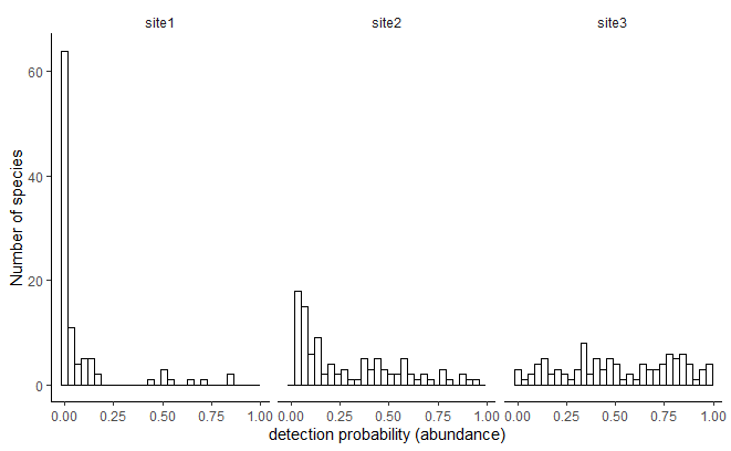
Then, for each of these three sites I will simulate sampling events. For each sampling event I draw the number of detections for each species in a Binomial distribution, \(B(t,p)\), where \(t\) is the number of trials (a proxy for the sampling intensity) and \(p\) the detection probability of the species. I simulate 10 replicates for different values of sampling intensity and number of sampling events. For each simulations I used the iNEXT R function to estimate the asymptotic richness. Below is the code of the simulations, with some dirty nested loops and rbinds.
library(reshape2)
library(iNEXT)
# a vector of different sampling effort
samp_vec =c(1,3) #sampling intensity
samp_events=c(5,10,20) #number of sampling events

# generate the records
nbrep=10
resf=NULL
for(si in unique(sp_pool$site)){ #loop over site
    pool=subset(sp_pool,site==si)
    for(ii in samp_vec){ #loop over sampling intensity
        for(i in samp_events){ #loop over different number of sampling events
            for(z in 1:i){ # generating sampling events
                for(j in 1:nbrep){ #loop over replicates
                    vec=c(sapply(pool$prob,function(x){rbinom(1,ii,x)}))
                    resf=rbind(resf,data.frame(sp=rep(pool$sp,vec),samp=ii,nbsamp=i,samp_event=z,site=si,rep=j))
                }
            }
        }
    }
}


b=resf %>% group_by(samp,site,rep,sp,nbsamp,samp_event) %>% count(name ="abund") #aggregate data per species, for each site and simulation parameters

b$id=paste(b$site,b$rep,b$nbsamp,b$samp,sep=".") #create a unique id for each simulations

comm=split(b, b$id) #creat a list fo community data, one dataframe per simulations
comm=lapply(comm,function(x){dcast(x,id+sp~samp_event,value.var="abund",fill=0)}) #put each data frame in the right format for iNEXT function
comm=lapply(comm,function(x){x[,-c(1:2)]}) #remove id columns

rari=iNEXT(comm,q=0,size=c(50,100,500,1000),datatype ="incidence_raw")
Once this is done, let’s have a look at the results.
rich_out=subset(rari$AsyEst,Diversity=="Species richness") #extract the predicted richness
rich_out=merge(rich_out,unique(b[,c("id","site","samp","rep","nbsamp")]),by.x="Assemblage",by.y="id") #adding information about parameters of simulations to that

pl2=ggplot(data=rich_out,aes(x=as.factor(nbsamp),y=Estimator,color=as.factor(samp)))+geom_boxplot()+xlab("Number of sampling events")+ylab("Richness estimation")+
theme_bw()+theme(axis.line = element_line(colour = "black"),panel.grid.major = element_blank(),panel.grid.minor = element_blank(),panel.background = element_blank(),plot.title=element_text(size=14,face="bold",hjust = 0),
strip.background=element_rect(fill=NA,color=NA),panel.border=element_blank(),legend.position="right")+labs(color="Sampling intensity")+
facet_wrap(~site)+geom_hline(aes(yintercept=nbsp))

pl2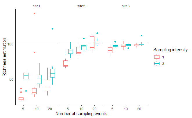
The estimated richness depends on the abundance distribution, which is fair, because the site with an exponential distribution of abundances have a significant amount of rare species, that could almost be considered as not present. More problematic, is that the predicted richness depends on sampling pressure. If for uniform distribution (site 3) the method corrected well for sampling effort, it was not the case for more uneven abundance distributions (sites 1 & 2).
It seems that having too many rare species make increases the uncertainty of the estimation (boxplots are wider in site 1) and make the method inefficient to correct by the sampling pressure. Abundance distributions appear to be strongly uneven in nature (callaghan2023?), with quite a high proportion of rare species, so this seems to be a real issue.