Occupancy models with INLA misestimate occupancy

Summary

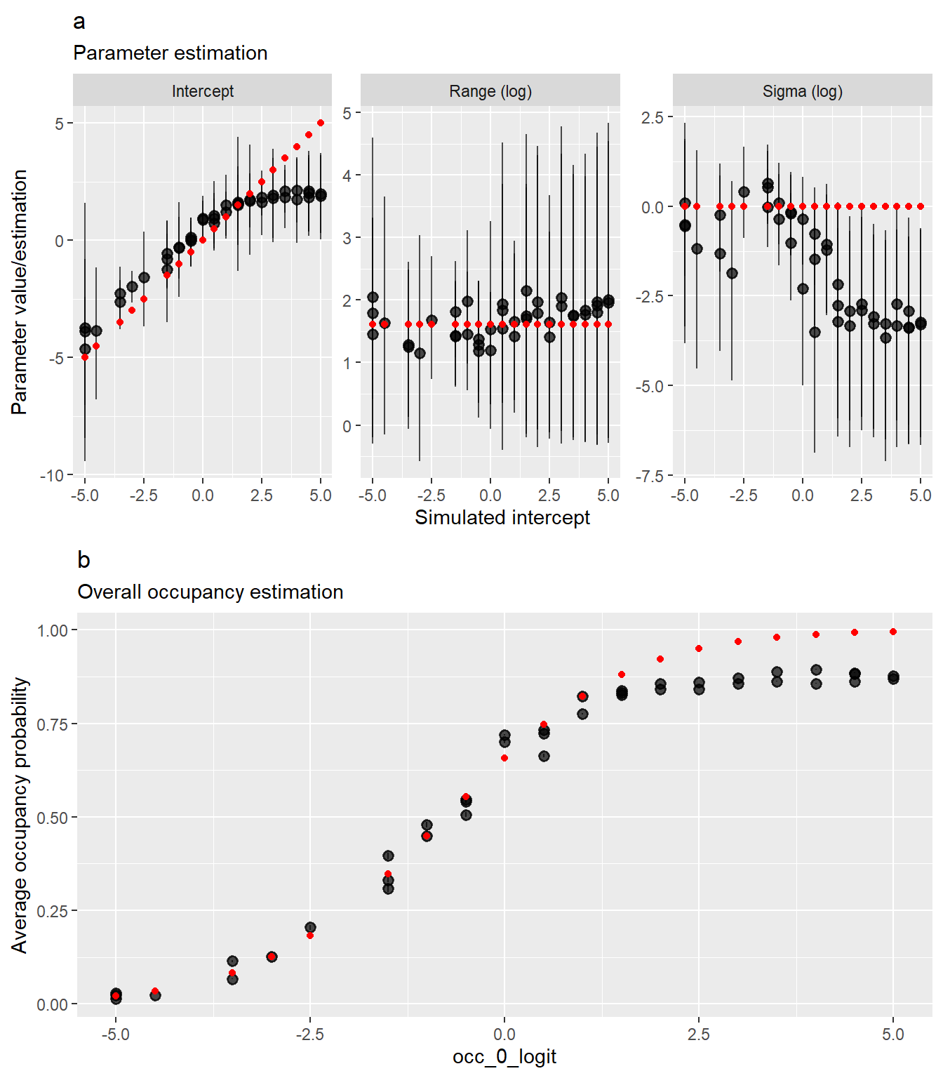
We have coded occupancy models using the very nice available tutorials and they have been working fine so far. However, when simulating datasets with a high occupancy probability we observe that INLA models gave completly wrong estimates of the intercept and other parameters associated with the spatial field. Below you will find a code allowing to reproduce that bug. This code simulates datasets with different intercepts and assess parameters’ estimation by INLA occupancy models.

The occupancy model

The occupancy model we will run here is a very simple model: a single year occupancy model with just a baseline detection probability in the observation model and an intercept + a spatial field in the state model.

State model

\[z_{i} \sim \mathrm{Bernoulli}(\psi_{i})\] \[\operatorname{logit}(\psi_{i}) = \beta_0 + \omega_i\] Observation model
\[y_{ij} \mid z_{i} \sim \mathrm{Bernoulli}(z_{i}\times p_{ij})\] \[ \operatorname{logit}(p_{ij}) = \alpha_0 \]

Here, \(z_{i}\) denotes the occupancy state in site \(i\). \(\psi_{i}\) is the associated occupancy probability defined on the logit scale as a linear function of an intercept (\(\beta_0\)) and \(\omega\), a spatial Gaussian random field describing the spatial structure in the data.

The response \(y_{ij}\) is the detection/non-detection data for site \(i\) and visit \(j\), given \(z_{i}\). The detection probabilities \(p\) are defined on the logit scale as a linear function of \(\alpha_0\) (Intercept).

The problem

In our simulation scenario, we simulated a spatial field of occupancy (on the logit scale) and we varied the intercept on that logit scale (\(\beta_0\)). This is supposed to be a simple easy case of estimation for the model, because even if we have only one year, thus one realization of the Bernouilli processes, we sample all sites of the studied area, thus we do not unsampled areas. In most of the cases model estimations were ok. However, when increasing \(\beta_0\) above a given threshold (\(\beta_0 > 2\), which means \(\psi \approx 0.88\) ) then we observe that the model estimation degraded very quickly to become very bad.

R and INLA versions

Loading packages and showing R and INLA versions:

library(data.table)
library(INLA)
library(fmesher)
library(raster)
library(dplyr)
library(sf)
library(terra)
library(spatstat.geom)
library(MASS)
library(ggplot2)
library(cowplot)

R.version

               _                                
platform       x86_64-w64-mingw32               
arch           x86_64                           
os             mingw32                          
crt            ucrt                             
system         x86_64, mingw32                  
status                                          
major          4                                
minor          5.2                              
year           2025                             
month          10                               
day            31                               
svn rev        88974                            
language       R                                
version.string R version 4.5.2 (2025-10-31 ucrt)
nickname       [Not] Part in a Rumble           

packageVersion("INLA")

[1] '26.9.17'

Simulating data

We first define an arbitrary spatial domain to simulate a spatial field representing variation in occupancy on the logit scale. Then we draw presences from that occupancy layer and detection and non-detection for each simulated visit. We then fitted the occupancy model using these detection and non-detection events only, to see the model could retrieve the simulated occupancy layer.

#Simulations parameters
nc <- 20 #number of grid cells acros latitude
nr <- 20 #number of grid cells acros longitude, 20*20 means 400 sites
nM <- 51 #maximal number of repeated visits, let's say 51 if we aggregate data at week level
occ_0_logit <- 0 #intercept of the model
det_prob <- 0.2 #detection probability
nrep_avg <- 5 #average number of repeated visits (1 repetition means 2 visits in a year per site)
# Range and sigma0 define the spatial field:
sigma0 <- 1 
range0 <- 5
nrepli <- 3 #number of replicate per simulation scenario

# Define spatial domain
win <- owin(c(0,10), c(0,10))

Domain <- rast(nrows=nr, ncols=nc,
               xmax=win$xrange[2],xmin=win$xrange[1],
               ymax = win$yrange[2],ymin=win$yrange[1])

values(Domain) <- 1:ncell(Domain)
names(Domain)="cell_id"

# 1. Define a spatial domain and create a mesh
locs <- crds(Domain) # 500 random points in a 10x10 square
mesh <- inla.mesh.2d(locs, max.edge = c(0.75, 2), cutoff = 0.5)
# 2. Build the SPDE model (Matérn covariance)
spde <- inla.spde2.matern(mesh = mesh, alpha = 2)
# 3. Compute the precision matrix (Q) for the SPDE model
# Kappa and tau can be derived from range0 and sigma0
kappa0 <- sqrt(8) / range0
tau0 <- 1 / (sqrt(4 * pi) * kappa0 * sigma0)
Q <- inla.spde2.precision(spde, theta = c(log(tau0), log(kappa0)))
spatial_field <- inla.qsample(n = 1, Q = Q)
spatial_values <- as.vector(spatial_field[mesh$idx$loc, ])

#let's generate many different datasets with different intercepts
data_list=list()
n <- 0
for(occ_0_logit in seq(-5,5,by=0.5)){
  for(j in 1:nrepli){
    n <- n+1
    #Now we can fit a model to that 
    tab=as.data.frame(Domain,xy=TRUE)
    tab$field=spatial_values
    tab$occ_0_logit=occ_0_logit
    tab$occupancy_logit=occ_0_logit+spatial_values
    tab$occupancy=boot::inv.logit(tab$occupancy_logit)
    tab$presence=rbinom(size=1,n=nrow(tab),prob=tab$occupancy)
    tab$nrep=1+rnbinom(nrow(tab),mu=nrep_avg,size=5)
    tab$nrep[tab$nrep>=nM]=nM
    tab$repli=j
    
    det_tab=do.call("rbind",lapply(1:nrow(tab),
                function(x){do.call("rbind",replicate(tab$nrep[x], tab[x,],simplify=FALSE))}))
    
    det_tab$rown=1:nrow(det_tab)
    
    det_tab = det_tab %>% dplyr::group_by(cell_id) %>% dplyr::mutate(Visite = seq_along(nrep))
    
    det_tab$detection=det_tab$presence*rbinom(nrow(det_tab),1,det_prob)
    
    
    matrix_spat=dcast(setDT(det_tab),cell_id+x+y+occupancy_logit+occupancy+presence+occ_0_logit+repli~paste0("W",Visite),value.var="detection")
    data_list[[n]]=matrix_spat
  }
}

Fitting the model

Now let’s fit the model for each of the simulated dataset, with different intercepts:

mesh_diameter <- max(diff(range(mesh$loc[,1])), diff(range(mesh$loc[,2]))) 
r_0 <- mesh_diameter/3 # Start with 1/3 of the total extent

spde <- inla.spde2.pcmatern(mesh = mesh,
                              prior.range = c(r_0,0.5),
                              prior.sigma = c(1, 0.5)) #start with the good values

# index set; "spatialfield" is the name used in the model formula
iset_sp <- inla.spde.make.index(name = "spatialfield", 
                                n.spde =  spde$n.spde)
model_list=list()
for(n in 1:length(data_list)){
  matrix_spat=data_list[[n]]
  # projection matrix using the coordinates of the data and time index
  A_sp <- inla.spde.make.A(mesh = mesh,
                         loc = as.matrix(matrix_spat[,c("x","y")]))
  
  #small mess to put detection covariates in the good format:
  Y_mat <- matrix_spat %>%
            dplyr::select(num_range("W",sort(unique(det_tab$Visite)))) %>% 
            as.matrix()
  matrix_spat$intercept=1
  
  #detection covariates in the good format (only one intercept):
  matrix_spat$intercept=1
  X_det <- matrix_spat[,rep("intercept",length(unique(det_tab$Visite))),with=FALSE] %>% as.matrix()
  
  #occupancy covariates
  X_cov <- matrix_spat %>%
  dplyr::select(c(cell_id))
  
  stk <- inla.stack(data=list(Y = Y_mat,  X = X_det),
                      A=list(A_sp,1),
                      effects=list(c(list(Int_occ=1), #the Intercept
                                     iset_sp),  #the spatial index
                                   #the covariates
                                   as.list(X_cov)),
                      tag='spat')
                      
  
  formula_spat <- inla.mdata(Y,X) ~ -1 + Int_occ +  f(spatialfield, model=spde)
  
  model_spat <- tryCatch({inla(formula_spat, data=inla.stack.data(stk),
            family= 'occupancy',
                    control.predictor=list(A=inla.stack.A(stk),compute=TRUE),
                    control.family = list(control.link = list(model = "logit"),
                    link.simple = "logit"),control.compute=list(config = TRUE,
                    waic=TRUE,cpo=TRUE,dic=TRUE,residuals=TRUE,mlik=TRUE))},
                    error=function(x){return(NA)})
  if(class(model_spat)=="inla"){
    model_list[[n]]=model_spat
  }
}

Assessing the fit

Now we can compare the simulated and model’s estimation for the parameters that defined occupancy (the intercept and the spatial field parameters):

pred_list=list()
est_list=list()

for(n in 1:length(model_list)){
  model_spat=model_list[[n]]
  matrix_spat=data_list[[n]]
  occ_0_logit=unique(matrix_spat$occ_0_logit)
  repli=unique(matrix_spat$repli)
  if(!is.null(model_spat)){
    field.result <- inla.spde2.result(
         inla = model_spat,        # Your fitted inla object
         name = "spatialfield", # Name of the SPDE spatial field component in your formula
         spde = spde,         # The spde object used in the model
         do.transf = TRUE     # Transform parameters back to nominal scale
    )
    
    est_fit=rbind(as.data.frame(model_spat$summary.fixed),field.result$summary.log.range.nominal[,-1],field.result$summary.log.variance.nominal[,-1])
    est_fit$variable=row.names(est_fit)
    est_fit$true_val=c(occ_0_logit,log(range0),log(sigma0))
    names(est_fit)[3:5]=c("lwr","median","upr")
    est_fit$occ_0_logit=occ_0_logit
    est_fit$repli=repli
    
    samples_spat = inla.posterior.sample(100, model_spat)
    post_val=do.call(cbind,
                  lapply(samples_spat,
                    function(X) X$latent[startsWith(rownames(X$latent), "APred")]))
    
    ## gather predictions together
    pred_df=matrix_spat %>%
                dplyr::select(c(names(X_cov),x,y,occupancy,occ_0_logit,occupancy_logit,presence,repli))
    pred_df$occupancy_est <- apply(post_val,1,mean)
    pred_df$sde <- apply(post_val,1,sd)
    pred_df$lwr <- apply(post_val,1,quantile,prob=0.025)
    pred_df$upr <- apply(post_val,1,quantile,prob=0.975)
    pred_list[[n]]=pred_df
    est_list[[n]]=est_fit
  }
}

pred_df=rbindlist(pred_list)
est_df=rbindlist(est_list)

Plot the fit for the models that did not crash only (might be incomplete if many models crashed):

p1=ggplot(data=est_df,aes(x=occ_0_logit,y=mean))+
  geom_pointrange(aes(ymin=lwr,ymax=upr),alpha=0.7)+
    geom_point(aes(y=true_val),color="red")+
  ylab("Parameter value/estimation")+
  xlab("Simulated intercept")+
  ggtitle("a",subtitle="Parameter estimation")+
  facet_wrap(~variable,scales="free_y",labeller=labeller(variable = c(Int_occ="Intercept",
                  range.nominal.1="Range (log)",variance.nominal.1="Sigma (log)")))

        
p3=ggplot(data=pred_df,aes(x=occ_0_logit,group=repli))+
    stat_summary(aes(y=boot::inv.logit(occupancy_est)),color="black",alpha=0.7)+
  stat_summary(aes(y=occupancy),color="red",geom="point")+
  ylab("Average occupancy probability")+
  ggtitle("b",subtitle="Overall occupancy estimation")

plot_grid(p1,p3,align="hv",ncol=1)

Red dots shows the simulated values while black points (& error bars) show the average estimation from the INLA models.