Occupancy Trends of European Pollinators
Ignasi Bartomeus 
François Duchenne
Carlos Martinez Nuñez
Abstract
This document present the dataset, methods and results of the SAFEGUARD project that aims to assess pollinator temporal trends at European level. First, we present the dataset and the associated challenges to succeed to unravel the population trends of european pollinators from opportunistic data that have not been collected for that. Second, we present how we used occupancy models to overcome possible bias. Third, we present the preliminary results of these model, showing the occupancy trends for ~480 species and comparing the 5 major biogeographic regions of Europe.
1 Dataset
The dataset is essentially composed from the database assembled by Natasha de Manincor et al. completed by a more recent version of the Iberian dataset (Bartomeus comm. pers.) and recently available dataset of bee occurrences from Portugal (https://doi.org/10.15468/2e4rap).
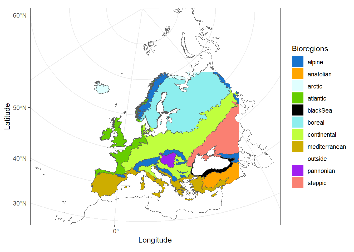
The merged dataset contains 4,921,255 records of pollinator occurrences between 1921 and 2020, within the region symbolized by the colored region in Figure 1.
We focused on the 5 biogeographic regions gathering most of the occurrence records, removing 93,254 records, leading to a dataset of 4,828,001 pollinator occurrences.
2 Methods to estimate occupancy trends
2.1 Inference of non-detection events
Because opportunistic data are composed only from presence data, we need to infer pseudo-absences, or non-detection events, to inform statistical models about potential absences. To do so, we need to define sites and survey events. Site were defined as grid cells, data being aggregated spatially using the hexagonal grid cells of side of 50km, which leads to grid cells of 6495km2. In a given site, records were grouped in survey events, by year and month. We defined a species’ detections in survey as the collection of the observed species at this location and during that survey. Conversely, we defined non-detections for a species if it was not observed at a given site during a given survey. This led to the exclusion of all records without information of the month of the collect (n = 1,919,779). We also removed the sites that had been surveyed only in one year (n = 325), because they do not bring temporal information, and their removal have been shown to improve modelling performance (Isaac et al. 2014). This led to 133,413 survey across the study area, between 1921 and 2020 (Figure 2).
This dataset is bias toward western Europe, Belgium and Soutern UK being the region with the better temporal coverage (Figure 2).
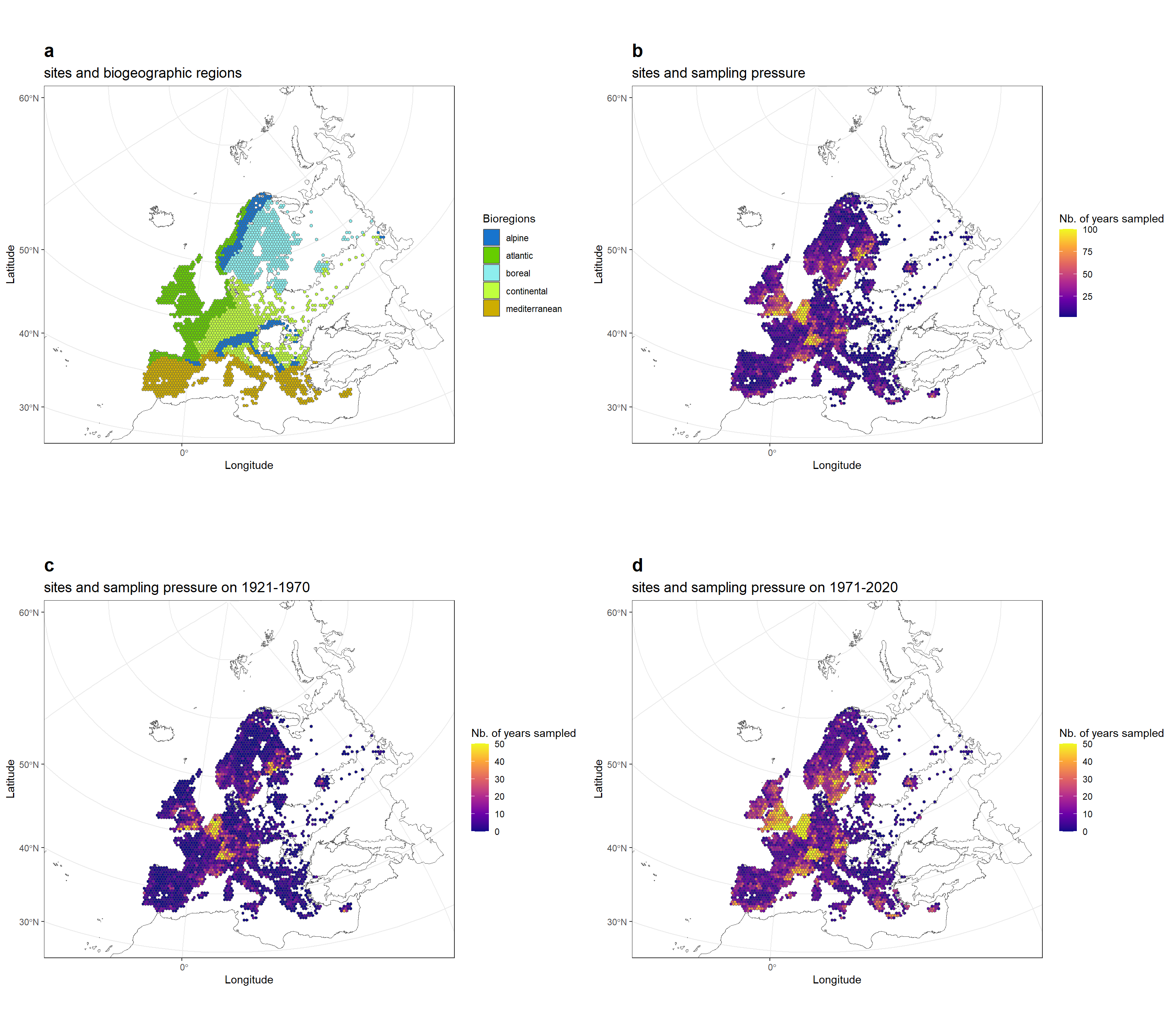
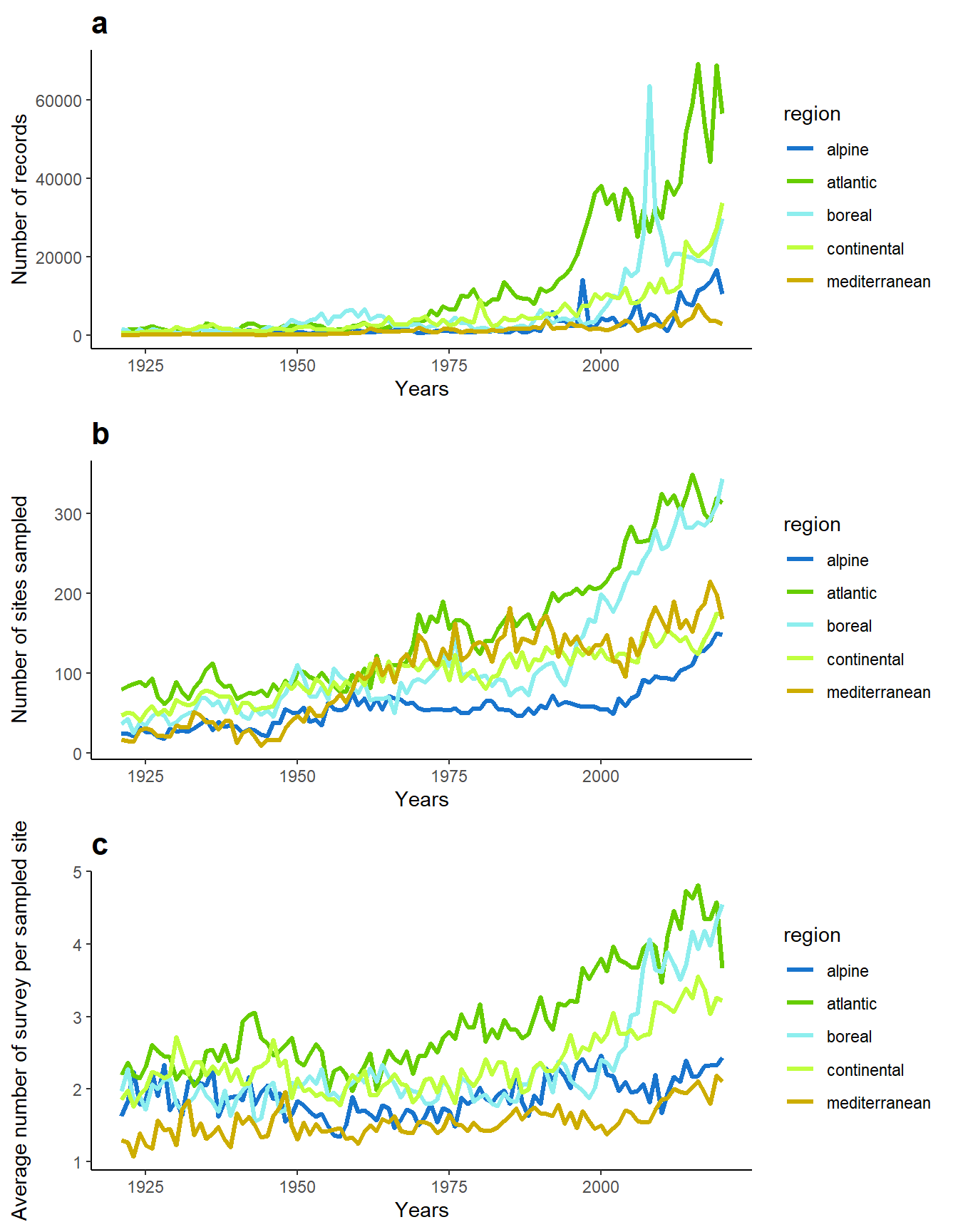
The dataset is also strongly temporally biased, with a sampling pressure that increased a lot over time, in terms of number of records, sites sampled and number of survey per sampled site (Figure 3).
2.2 Statistical model
The corrections of these bias require the use of statistical models that distinguish the observation processes and the population states. To do so we used occupancy models, which have been shown as one of the most powerful methods to estimate population trends from opportunistic data (Isaac et al. 2014; Outhwaite et al. 2019; Shirey et al. 2023). This method accounts for temporal variation in detection probability, thereby considering changes over time in the species targeted by collectors. Temporal variation in occupancy measured at broad spatial scale is considered as a proxy of population trend, due to the close relationship between abundance and occupancy (He and Gaston 2003).
To see how model formulation could affect our results, we run two different models: one modelling linear temporal changes in occupancy and another one modelling non-linear temporal changes in occupancy. Linear trends are convenient because they allow to resume in one coefficient (the slope) if the direction and the magnitude of the population trend. However, summarizing non-linear variation to a linear trends can lead to biased trends (Duchenne et al. 2022), which thus require to assess the linearity of the studied temporal changes to draw relevant conclusions.
2.2.1 Linear temporal changes in occupancy
The model was fitted independently for each species, and described by the following set of equations:
State model:
\[ z_{rij} \sim Bernouilli(\Psi_{rij}); logit(\Psi_{rij})=\beta_0 + \tau_r \times year_j + \Theta_i \tag{1}\]
Observation model:
\[ \begin{align} y_{rijv} | z_{rij} &\sim Bernouilli(p_{rijv} \times z_{rij}); \\ logit(p_{rijv}) &=\beta_1 + \beta_2 \times sampling \space completeness_{ijv} + \Theta_{r,month_v}+ \Theta_{j} \end{align} \tag{2}\]
The state model describes the true (unknown) occupancy of the species (\(z_{rij}=0\), absent or \(z_{rij}=1\), present). \(\Psi_{rij}\) is the probability of occupancy in region r, grid cell i at year j. This probability is modeled using a logit link function, as a function of a global intercept \(\beta_0\), a fixed linear effect of the time for each region r (\(\tau_r\)) and a random site effect (\(\Theta_{i}\)).
The observation model describes detection/non-detection events in region r, grid cell i, time period j, and survey v (\(y_{rijv}\)), conditionally to the true occupancy state (\(z_{rij}\)). It models the detection status of the focal species (1 or 0) . \(p_{rijv}\) is the estimated detection probability, modelled as a function of an intercept \(\beta_1\), a fixed effect (\(\beta_2\)) of the sampling completeness.Our measure of sampling completeness was simply the logarithm of the number of species detected during survey v. This index was centered per region to remove the correlation with regional species richness. Because we log transformed the number of species detected, this effect captures whether during a survey, one, few or more species were detected, which mainly depends on the sampling pressure (Isaac et al. 2014).
Finally, to the observation model, we added a nested random effect of the month on of the survey v within the region r (\(\Theta_{r,month_v}\)) to model phenological variation in detection probability across months and regions, and a random effect of the year (\(\Theta_j\)) to absorb temporal variation in detection probability of the focal species.
When using a linear temporal trend and a logit function, it has been shown that the slope of that temporal trend (\(\theta_r\)) is the logarithm of the growth rate (\(\rho\)) (Duchenne et al. 2022). Thus \(\rho_r=e^{\theta_r}\), where \(\rho=1\) means a stale occupancy probability, \(\rho<1\) a decrease and \(\rho>1\) a temporal increase in occupancy probability. To get a more intuitive measure of growth rate, we decided to express this growth rate in \(\pm \%.year^{-1}\) we used: \(\rho_r=100 \times (e^{\theta_r}-1)\).
2.2.2 Non-linear temporal changes in occupancy
The non-linear model was exactly the same as the linear model presented in Equation 1 and Equation 2, excepting that we replaced the linear temporal trend for each region r (\(\tau_r\)) in Equation 1 by an autoregressive process of order 1 (AR1, \(\Theta_{rj}\)), leading to the following state model:
State model:
\[ z_{rij} \sim Bernouilli(\Psi_{rij}); logit(\Psi_{rij})=\beta_0 + \Theta_{rj} + \Theta_i \tag{3}\]
2.2.3 Model implementation
Considering the important size of our dataset, due to the broad spatio-temporal scales considered here, we decided to implement our model using the R package glmmTMB to take adavantage of the fast computation it offers, instead of heavier and slower bayesian implementations (Isaac et al. 2014). To do so, we implemented the state model in the zero inflation formula. For example for the linear model, it was coded as follow:
model=glmmTMB(Y~sampling_completeness+(1|year)+(1|region/month),ziformula=~year*region+(1|site),family=binomial,data=dat)We fitted this model for all species with at least 10 records in Europe, and that have been detected in at least 5 surveys in a given region. For each species, we removed the biogeographic regions in which the species has been detected in less than 5 surveys. This led to a list of 1,332 species, over the 1,745 species in the dataset.
Since optimization of the model was tricky, to maxmimize the chance of convergence, we tried 4 different solvers compatible with glmmTMB: nlimb, Nelder-Mead, BFGS and CG. We also tried two different covariance structures for the temporal autocorrelation in the non-linear occupancy model: AR1 and the Ornstein-Uhlenbeck. We run models in the order listed in the Table 1 and kept the first model that converged.
| solver | covariance structure | order of run |
|---|---|---|
| nlimb | AR1 | 1 |
| Nelder-Mead | AR1 | 2 |
| BFGS | AR1 | 3 |
| CG | AR1 | 4 |
| nlimb | Ornstein-Uhlenbeck | 5 |
| Nelder-Mead | Ornstein-Uhlenbeck | 6 |
| BFGS | Ornstein-Uhlenbeck | 7 |
| CG | Ornstein-Uhlenbeck | 8 |
3 Results
3.1 Species with convergence problems
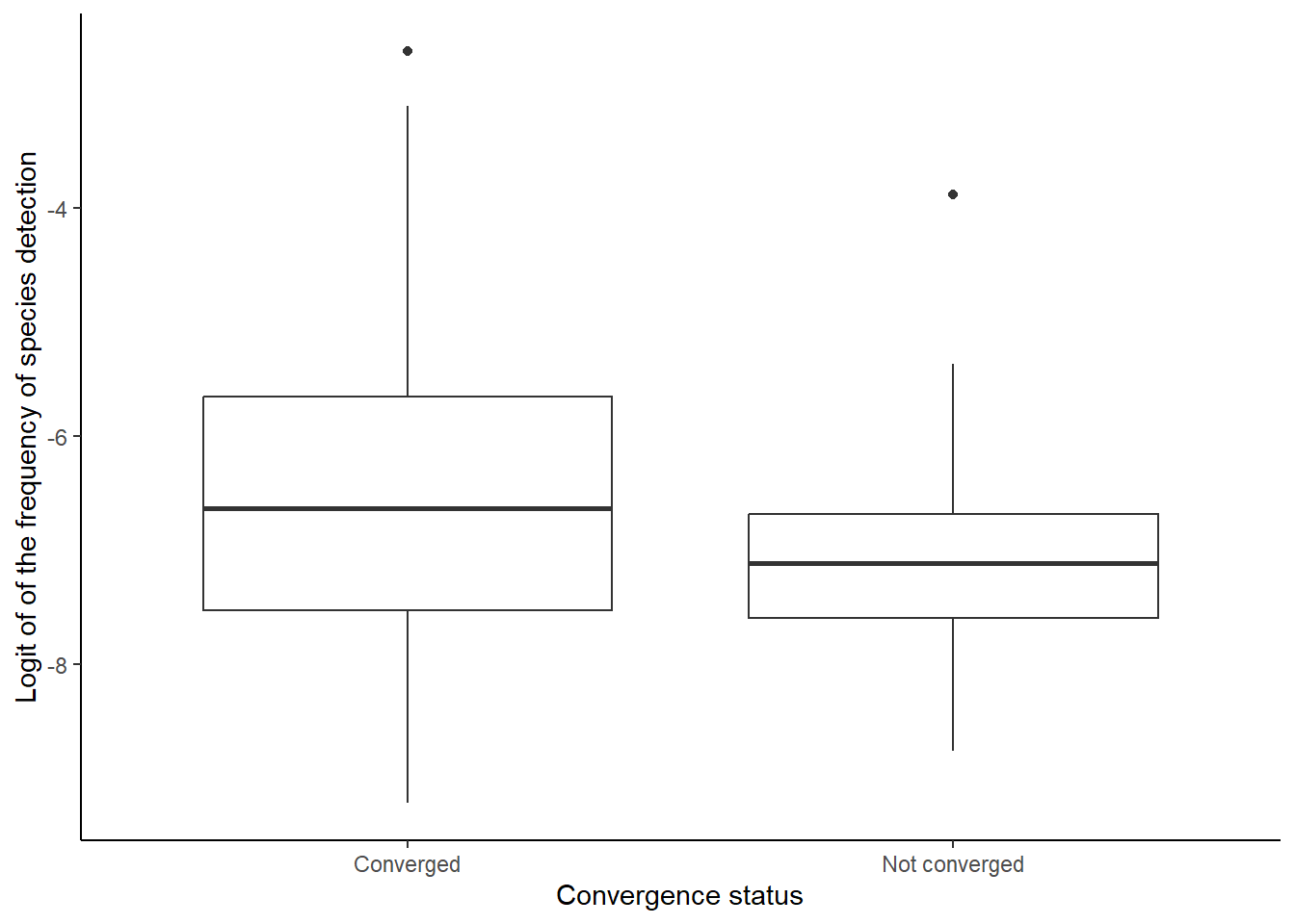
For 854 species, occupancy trends could not be estimated properly because the model did not converge, regardless the algorithm used to optimize the model (“nlimb”, “Nelder-Mead”, “BFGS” or “CG”). Most often these convergence problems are due to positive values in the Hessian Matrix, likely due to a flat likelihood profile. This means that a broad diversity of parameter combination are consistent with the observations, and thus that the data do not contain enough information to infer spatio-temporal patterns of occupancy in a reliable way. These problems of convergence tended to occur slightly more often when the species was detected in very few surveys (i.e. rare species, Figure 4). This is a bias that our study, and other similar studies have faced (Duchenne et al. 2020; Powney et al. 2019): we do not have enough historical data to model occupancy trends of the species that became rare or extinct before recent times. Thus our occupancy trends do not include these strong historical declines that are likely an important components when estimating the effect of past global change on biodiversity. This is a source of under-estimation of effects of global change on biodiversity that is important to keep in mind.
These problems of convergence might be possible to solve in the future, by subsampling the dataset to focus on the core of the species area only, but it is for now a work in progress. It would also make the comparison across species slightly more difficult.
3.2 Linear occupancy trends
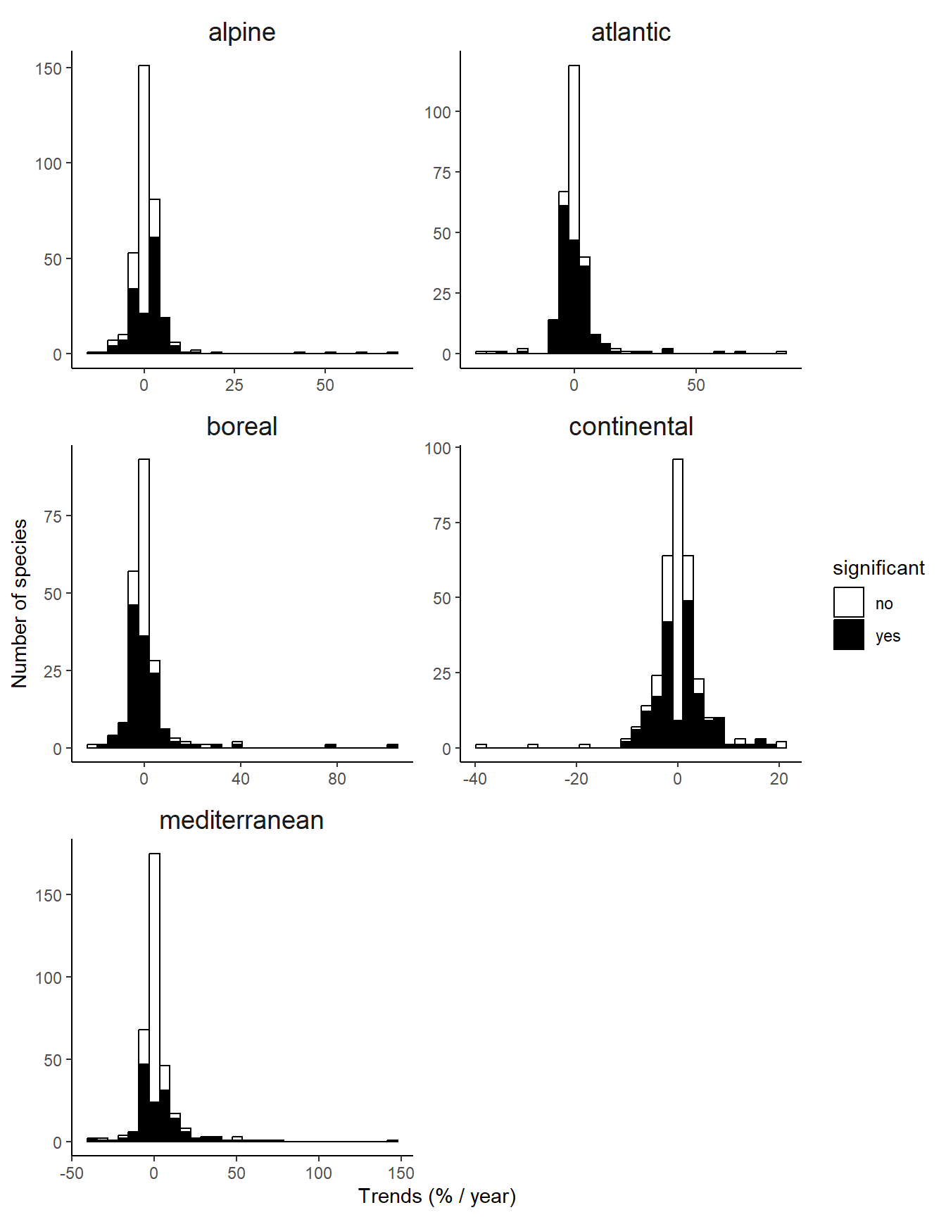
We were able to estimate the occupancy trends for 478 species, for a total number of 1493 population trends, for each possible species-region combinations. Among those combinations, 4 population trends were excluded from the dataset because they presented extreme values (positive or negative,\(|\tau_r|>1\)) that are likely to be erroneous trends.
The occupancy trends estimated for the remaining 1489 combination of species and biogeographic regions show a mixture of winners (species significantly increasing in occupancy, 27.94%) and losers (species significantly decreasing in occupancy, 25.25%) of the past global change (Figure 5).
The distribution of occupancy trends tended to be skewed on the right, with few very positive occupancy trends, suggesting the colonization of new area by some species, which is a typical signature of global change-driven changes.
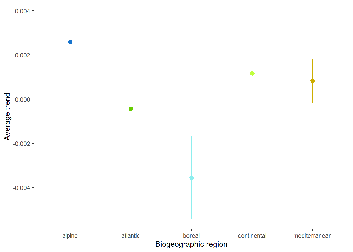
Calculating the arithmetic mean of these occupancy trends per region we observe an average decline only in the Atlantic bio-geographic region (Figure 6). It is however important to note the strong uncertainty around these average values, due to the heterogeneity in occupancy trends across species.
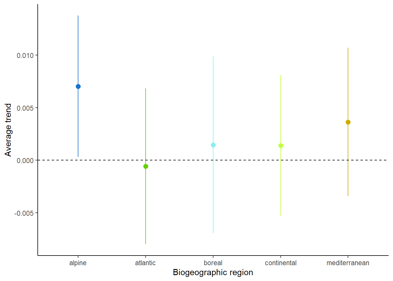
Moreover, although most of the region exhibit a positive average occupancy trend, this positive trend is driven by the right-skewness of the distribution (Figure 5). When looking at the proportion of losers and winners per region, losers are often as common as winners (Table 2). The only exception is the alpine biogeographic region, in which winners are strongly over-represented. This is consistent with the expectations under a climate warming scenario (Pradervand et al. 2014).
| Region | Proportion of losers | Proportion of winners |
|---|---|---|
| alpine | 0.15 | 0.31 |
| atlantic | 0.39 | 0.28 |
| boreal | 0.33 | 0.30 |
| continental | 0.25 | 0.30 |
| mediterranean | 0.20 | 0.22 |
3.3 Non-linear occupancy trends
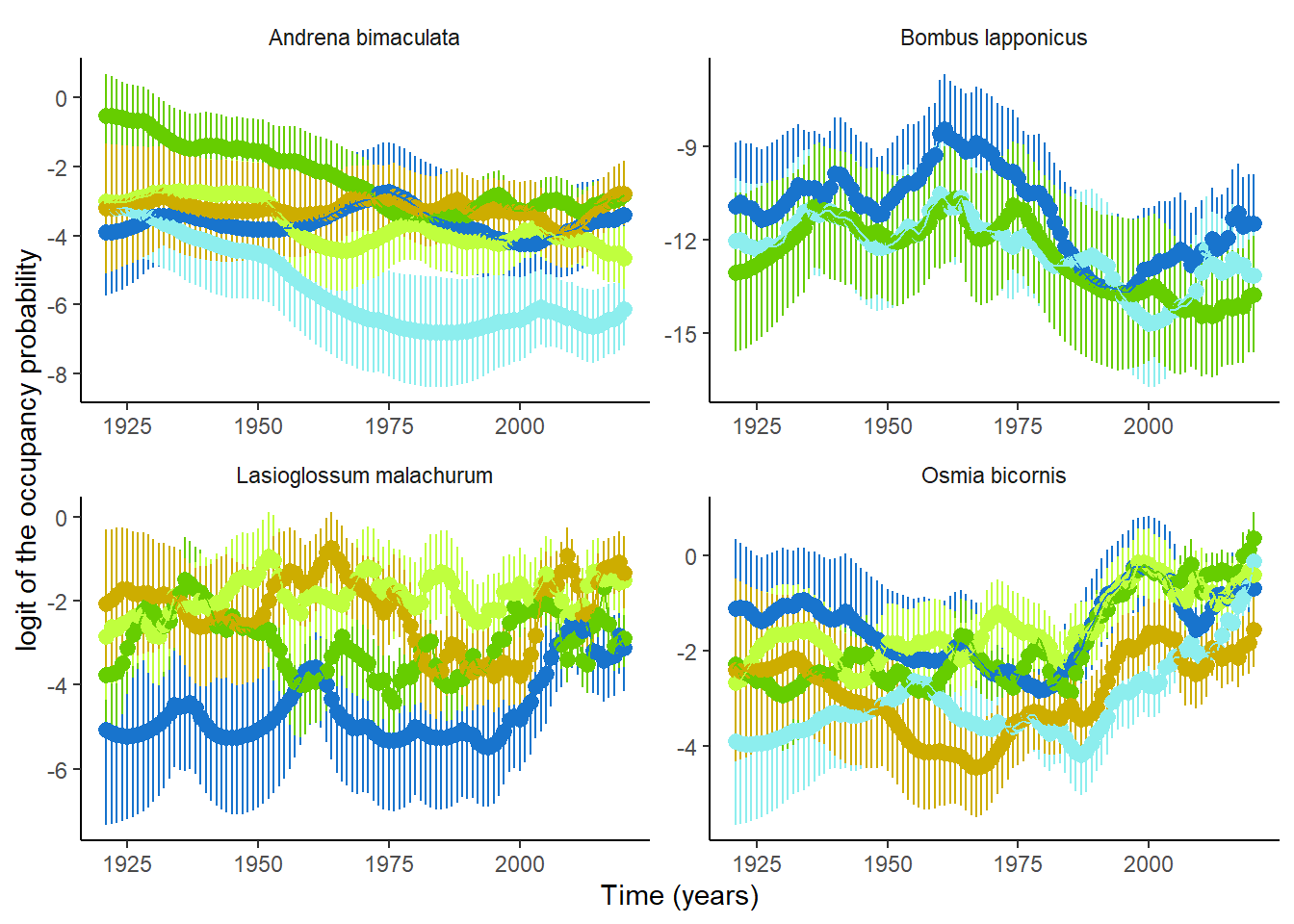
Using the second kind of occupancy model, accounting for non-linearity, described in Section 2.2.2,we could exemplify that occupancy trends are indeed rarely linear (Figure 7).
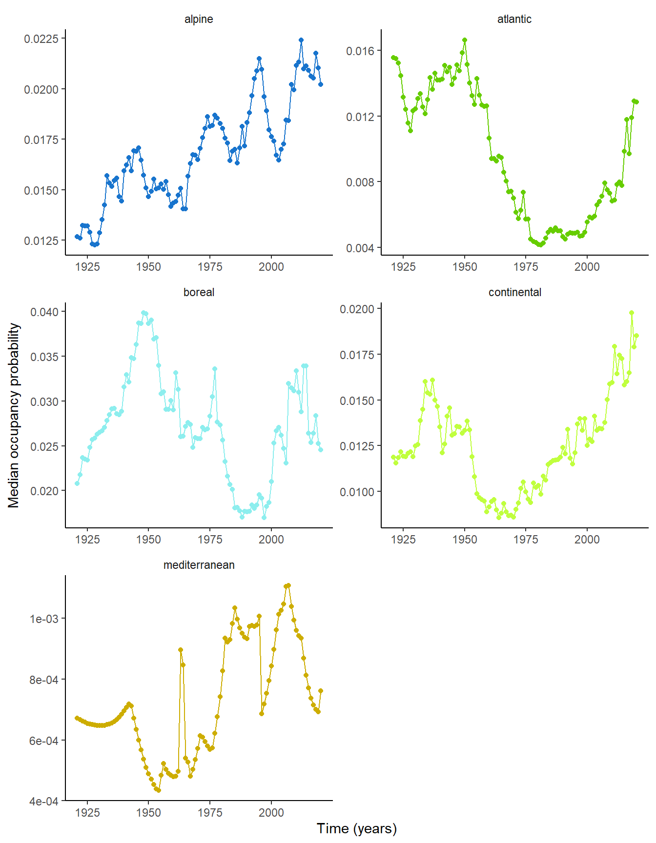
When looking at how the median of the occupancy probability varies over time, we notice an historical decline in the Boreal, Continental and Atlantic regions, followed by a recent increase in occupancy probability, in a “U” shaped pattern that is consistent with what we know from other studies (Duchenne et al. 2020; Carvalheiro et al. 2013). In contrast, alpine region shows a constant increase in median occupancy probability over-time. This is consistent with the displacement of species-rich lowlands bee communities towards higher elevation. Moreover, the fact that the Alpine region does not exhibit the “U” shaped temporal variation in occupancy observed in the Continental and Atlantic regions is consistent with the fact that this historical decline has been driven by agricultural intensification.
Finally, Mediterranean region shows a slight increase in median occupancy probability but the temporal pattern is rather unclear and variation is weak, probably due to the lack of historical data in that region.
We can use this model to retrieve linear temporal trends in occupancy across 1921-2020, but accounting for the uncertainty due to non-linearity, to compare results with previous ones. When looking at average occupancy trends per biogeographic regions we observe a result slightly different results than those presented in Section 3.2.
4 References
Carvalheiro, Luísa Gigante, William E. Kunin, Petr Keil, Jesus Aguirre‐Gutiérrez, Willem Nicolaas Ellis, Richard Fox, Quentin Groom, et al. 2013. “Species Richness Declines and Biotic Homogenisation Have Slowed down for NW-European Pollinators and Plants.” Ecology Letters 16 (7): 870–78. https://doi.org/10.1111/ele.12121.
Duchenne, François, Emmanuelle Porcher, Jean-Baptiste Mihoub, Grégoire Loïs, and Colin Fontaine. 2022. “Controversy over the Decline of Arthropods: A Matter of Temporal Baseline?” Peer Community Journal 2. https://doi.org/10.24072/pcjournal.131.
Duchenne, François, Elisa Thébault, Denis Michez, Maxence Gérard, Céline Devaux, Pierre Rasmont, Nicolas J. Vereecken, and Colin Fontaine. 2020. “Long-Term Effects of Global Change on Occupancy and Flight Period of Wild Bees in Belgium.” Global Change Biology 26 (12): 6753–66. https://doi.org/https://doi.org/10.1111/gcb.15379.
He, Fangliang, and Kevin J. Gaston. 2003. “Occupancy, Spatial Variance, and the Abundance of Species.” The American Naturalist 162 (3): 366–75. https://doi.org/10.1086/377190.
Isaac, Nick JB, Arco J. van Strien, Tom A. August, Marnix P. de Zeeuw, and David B. Roy. 2014. “Statistics for Citizen Science: Extracting Signals of Change from Noisy Ecological Data.” Methods in Ecology and Evolution 5 (10): 10521060.
Outhwaite, Charlotte L., Gary D. Powney, Tom A. August, Richard E. Chandler, Stephanie Rorke, Oliver L. Pescott, Martin Harvey, et al. 2019. “Annual Estimates of Occupancy for Bryophytes, Lichens and Invertebrates in the UK, 1970–2015.” Scientific Data 6 (1): 259. https://doi.org/10.1038/s41597-019-0269-1.
Powney, Gary D., Claire Carvell, Mike Edwards, Roger K. A. Morris, Helen E. Roy, Ben A. Woodcock, and Nick J. B. Isaac. 2019. “Widespread Losses of Pollinating Insects in Britain.” Nature Communications 10 (1): 1018. https://doi.org/10.1038/s41467-019-08974-9.
Pradervand, Jean-Nicolas, Loïc Pellissier, Christophe F. Randin, and Antoine Guisan. 2014. “Functional Homogenization of Bumblebee Communities in Alpine Landscapes Under Projected Climate Change.” Climate Change Responses 1 (1): 1. https://doi.org/10.1186/s40665-014-0001-5.
Shirey, Vaughn, Rassim Khelifa, Leithen K. M’Gonigle, and Laura Melissa Guzman. 2023. “Occupancy–Detection Models with Museum Specimen Data: Promise and Pitfalls.” Methods in Ecology and Evolution 14 (2): 402–14. https://doi.org/10.1111/2041-210X.13896.